Loggers and field equipment provide many different datasets format.
The readr::read_delim (Wickham
et al., 2024) function works perfectly in most cases,
given that the data are in a delimited file.
We provide here examples on how to use read_delim to
prepare your raw data files for the fluxible R package. For
users of Li-COR instruments, the licoread
R package, developed in collaboration with Li-COR, is designed to
read 82z and 81x files and import them as fluxible-friendly
objets.
Eosense ecosystem gas flux chambers users can also use the readosense R
package to read their raw files and import them as
fluxible-friendly objects.
Checklists for inputs
The first function to use when processing ecosystem gas fluxes data
with fluxible is flux_match, which requires
two inputs: row_conc and field_record. The
columns in both files do not require specific names, and those will be
kept during the entire workflow. We however advise that those names do
not contain spaces or special characters.
Input raw_conc
The input raw_conc is the file with the gas
concentration measured over time, typically the file exported by the
logger or instrument, and needs to fulfill the following criteria:
- A column with gas concentration as numeric values
- A column in datetime format (
yyyy-mm-dd hh:mm:ss) corresponding to each data point of gas concentration
Input field_record
The input field_record is the metadata file that
contains the information of when which sample or plot was measured. It
can also provide other meta data, such as campaign, site, type of
measurement, etc. This file should contain:
- A column indicating the start of each measurement in datetime format
(
yyyy-mm-dd hh:mm:ss) - If the length of the measurements is not a constant: a column
containing the end of each measurement in datetime format
(
yyyy-mm-dd hh:mm:ss)
By-passing flux_match
The flux_match function only intends to attribute a
unique flux_id to each measurement and slice out recordings
in between measurements. Depending on your setup, this step might not be
necessary. The flux_fitting function is the step after
flux_match and its input should check the following
points:
- A gas concentration column as numeric
- A column in datetime format (
yyyy-mm-dd hh:mm:ss) corresponding to each gas concentration data points - A column with a unique ID for each measurement
- A column indicating the start of each measurement in datetime format
(
yyyy-mm-dd hh:mm:ss) - A column indicating the end of each measurement in datetime format
(
yyyy-mm-dd hh:mm:ss)
Defining your dataset
fluxible treats the entire dataset homogeneously in
terms of choice of model to fit the data and quality control. This is
because every step in this process has a risk of adding a bias to the
final data (for example, a linear fit tends to under estimate fluxes
while an exponential one tends to over estimate fluxes). By treating the
data homogeneously, the bias are consistent and therefore will affect
further analysis less.
Measurements done under similar conditions and with the same equipment
should ideally be processed together.
Importing a single file
In this example we will import the file 26124054001.#00,
which is a text file extracted from a Squirrel Data Logger 2010 Series
(Grant Instruments) through SquirrelView software. The first thing to do
when importing a file with read_delim is to open the file
in a text editor to look at its structure.
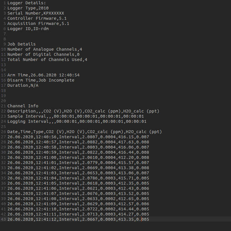
26124054001.#00 in a text editor. We can see that the 25th
first rows do not need to be imported, and that it is comma separated
with a dot as a decimal point.
We will read the file with read_delim, and then use
rename and mutate (from
the dplyr package ; Wickham et al., 2023)
to transform the columns into what we want, and dmy_hms
from the lubridate package (Grolemund and Wickham, 2011) to get our
datetime column in the right format:
library(tidyverse)
# readr, dplyr and lubridate are part of tidyverse

raw_conc <- read_delim(
  "ex_data/26124054001.#00",
  delim = ",", # our file is comma separated
  skip = 25 # the first 25 rows are logger infos that we do not want to keep
)
raw_conc structure:
#> spc_tbl_ [17 × 7] (S3: spec_tbl_df/tbl_df/tbl/data.frame)
#>  $ Date          : chr [1:17] "26.06.2020" "26.06.2020" "26.06.2020"..
#>  $ Time          : 'hms' num [1:17] 12:40:56 12:40:57 12:40:58 12:40..
#>  $ Type          : chr [1:17] "Interval" "Interval" "Interval" "Int"..
#>  $ CO2 (V)       : num [1:17] 2.08 2.09 2.08 2.08 2.06 ...
#>  $ H2O (V)       : num [1:17] 4e-04 4e-04 4e-04 4e-04 4e-04 4e-04 4e..
#>  $ CO2_calc (ppm): num [1:17] 416 418 416 416 412 ...
#>  $ H2O_calc (ppt): num [1:17] 0.007 0.008 0.007 0.008 0.008 0.007 0...
Not too bad… but we are not quite there yet:
- Some column names contain space
- Some columns are not needed, removing them will make things easier
later on:
Type(nothing to do with the type of measurement, something from the logger),CO2 (V),H2O (V)(those two are the voltage input to the logger, not needed), andH2O_calc (ppt)(that one was not calibrated for this campaign so better remove it to avoid confusion) - The
DateandTimecolumns should be united in one and transformed inyyyy-mm-dd hh:mm:ssformat
raw_conc <- raw_conc |>
  rename(
    co2_conc = "CO2_calc (ppm)"
  ) |>
  mutate(
    datetime = paste0(Date, Time), # we paste date and time together
    datetime = dmy_hms(datetime) # datetime instead of character
  ) |>
  select(datetime, co2_conc)
Et voilà:
#> tibble [17 × 2] (S3: tbl_df/tbl/data.frame)
#>  $ datetime: POSIXct[1:17], format: "2020-06-26 12:40:56" ...
#>  $ co2_conc: num [1:17] 416 418 416 416 412 ...
Importing multiple files
Quite often a field season will result in several files. In this example we will read all the files in “ex_data/” that contain “CO2” in their names.
library(tidyverse)

raw_conc <- list.files( # list the files
  "ex_data", # at location "ex_data"
  full.names = TRUE,
  pattern = "*CO2*" # that contains "CO2" in their name
) |>
  map_dfr(
    read_csv, # we map read_csv on all the files
    na = c("#N/A", "Over") # "#N/A" and Over should be treated as NA
  ) |>
  rename(
    conc = "CO2 (ppm)"
  ) |>
  mutate(
    datetime = dmy_hms(`Date/Time`)
  ) |>
  select(datetime, conc)
Units row below column names?
Some instruments include a row with units just below the column
names. This is annoying because read_delim will read that
row as data, and therefore the column with gas concentration will be
read as character instead of numeric. Normally, those units are stated
in the protocol or (draft) data paper of the project, so it is ok to
remove them. There are different ways to do that, here is one:
library(tidyverse)

co2 <- read_delim(
  "raw_data/NatuRA_raw_CO2_2026-01-18.data",
  skip = 5 # skipping the first 5 rows (instrument info)
  ) |>
  slice(-1) |> # we slice the first row (units)
  select(c(DATE, TIME, CO2)) |> # and select what we want
mutate(
  datetime = ymd_hms(paste(DATE, TIME)), # lubridate function to create datetime
                     CO2 = as.double(CO2),  # converting CO2 to numeric
                    .keep = "unused" # we remove DATE and TIME columns
                     )
The one file per flux approach
fluxible can also be used with data that were recorded
with one file per flux and the file names as flux ID. In that case,
flux_match can be skipped as we will directly import the
data with the flux IDs, and start and end of each flux measurements. In
this example we use the fluxible default column names to
make it easier for the rest of the data processing. The measurement
lengths are based on the start and end of the files, which might not be
accurate depending on the field routine. This can be adjusted with the
arguments start_cut, end_cut and
cut_direction in flux_fitting:
-
cut_direction = "none"(default) means the focus window is defined asstart + start_cuttoend - end_cut -
cut_direction = "from_start"means the focus window is defined asstart + start_cuttostart + end_cut -
cut_direction = "from_end"means the focus window is defined asend - start_cuttoend - end_cut
library(tidyverse)


raw_conc <- list.files( #listing all the files
  "ex_data/field_campaign", # at location "ex_data/field_campaign"
  full.names = TRUE
) |>
  map_dfr( # we map read_tsv on all the files
    # read_tsv is the version of read_delim for tab separated value files
    read_tsv,
    skip = 3,
    # creates a column with the filename, that we can use as flux ID
    id = "f_fluxid"
  ) |>
  rename( # a bit of renaming to make the columns more practical
    co2_conc = "CO2 (umol/mol)",
    h2o_conc = "H2O (mmol/mol)",
    air_temp = "Temperature (C)",
    pressure = "Pressure (kPa)"
  ) |>
  mutate(
    .by = f_fluxid,
    f_datetime = paste(Date, Time),
    # we get rid of the milliseconds
    f_datetime = as.POSIXct(f_datetime, format = "%Y-%m-%d %H:%M:%OS"),
    pressure = pressure / 101.325, # conversion from kPa to atm
    f_fluxid = basename(f_fluxid), # removing folder names
    f_start = min(f_datetime), # start is the smallest datetime of each flux
    f_end = max(f_datetime) # end is the greatest datetime of each flux
  ) |>
  select(
    f_datetime, co2_conc, h2o_conc, air_temp, pressure, f_fluxid, f_start, f_end
  )
raw_conc structure:
#> tibble [330 × 8] (S3: tbl_df/tbl/data.frame)
#>  $ f_datetime: POSIXct[1:330], format: "2023-12-14 10:57:01" ...
#>  $ co2_conc  : num [1:330] 416 407 404 421 411 ...
#>  $ h2o_conc  : num [1:330] 22.7 22.5 23 22.6 22.8 ...
#>  $ air_temp  : num [1:330] 22.4 22.4 22.4 22.3 22.3 ...
#>  $ pressure  : num [1:330] 0.79 0.791 0.79 0.79 0.791 ...
#>  $ f_fluxid  : chr [1:330] "1_2000_east_1_day_a-2023-12-14T105700.t"..
#>  $ f_start   : POSIXct[1:330], format: "2023-12-14 10:57:01" ...
#>  $ f_end     : POSIXct[1:330], format: "2023-12-14 10:58:48" ...
The tricky one
What happens when you extract a logger file in csv using a computer with settings using comma as a decimal point (which is quite standard in Europe)? Well, you get a comma separated values (csv) file, with decimals separated by… comma.
Ideally the file should have been extracted in European csv, which means comma for decimals and semi-colon as column separator. But here we are.
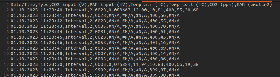
011023001.#01 opened in a text editor. We can see that it
is comma separated, but that the decimal point is also a comma.
Additionally, we see that some variables were measured only every 10
seconds, meaning that each row has a different number of commas…
Gnnnnnnn
Let’s try the usual way first:
library(tidyverse)

raw_conc <- read_csv( # read_csv is the same as read_delim(delim = ",")
  "ex_data/011023001.#01",
  col_types = "Tcdddddd",
  na = "#N/A" # we tell read_csv what NA look like in that file
)
#> spc_tbl_ [101 × 8] (S3: spec_tbl_df/tbl_df/tbl/data.frame)
#> $ Date/Time : POSIXct[1:101], format: NA ...
#> $ Type : chr [1:101] "Interval" "Interval" "Interval" "In"..
#> $ CO2_input (V) : num [1:101] 2 2 2 2 2 2 2 2 2 2 ...
#> $ PAR_input (mV): num [1:101] 28 28 28 35 31 23 58 35 7 3 ...
#> $ Temp_air ('C) : num [1:101] 0 NA NA NA NA NA NA NA NA NA ...
#> $ Temp_soil ('C): num [1:101] 80663 NA NA NA NA ...
#> $ CO2 (ppm) : num [1:101] 12 NA NA NA NA NA NA NA NA NA ...
#> $ PAR (umolsm2) : num [1:101] NA NA NA NA NA NA NA NA NA NA ...It took the column names right, but then of course interpreted all comma as separators, and made a mess. Let’s see if we can skipped the header and then assemble the columns with left and right side of the decimal point:
raw_conc <- read_csv(
  "ex_data/011023001.#01",
  skip = 1, # this time we skip the row with the column names
  col_names = FALSE, # we tell read_csv that column names are not provided
  na = "#N/A" # we tell read_csv what NA looks like in that file
)
#> spc_tbl_ [101 × 14] (S3: spec_tbl_df/tbl_df/tbl/data.frame)
#> $ X1 : chr [1:101] "01.10.2023 11:23:40" "01.10.2023 11:23:41" "01"..
#> $ X2 : chr [1:101] "Interval" "Interval" "Interval" "Interval" ...
#> $ X3 : num [1:101] 2 2 2 2 2 2 2 2 2 2 ...
#> $ X4 : chr [1:101] "0028" "0028" "0028" "0035" ...
#> $ X5 : num [1:101] 0 NA NA NA NA NA NA NA NA NA ...
#> $ X6 : chr [1:101] "080663" NA NA NA ...
#> $ X7 : num [1:101] 12 NA NA NA NA NA NA NA NA NA ...
#> $ X8 : chr [1:101] "00" "400" "400" "400" ...
#> $ X9 : chr [1:101] "10" "56" "55" "70" ...
#> $ X10: num [1:101] 81 NA NA NA NA NA NA NA NA NA ...
#> $ X11: num [1:101] 400 NA NA NA NA NA NA NA NA NA ...
#> $ X12: chr [1:101] "55" "" "" "" ...
#> $ X13: num [1:101] 20 NA NA NA NA NA NA NA NA NA ...
#> $ X14: chr [1:101] "60" "" "" "" ...The problem now is that CO2 concentration was measured every second (with a comma!), while other variable were measured every 10 seconds. That means every 10th row has 14 comma separated elements, while the others have only 10. Uhhhhhhhhh
At this point, you might want to get the field computer out again and re extract your raw file with a European csv output, or anything that is not comma separated, or set the decimal point as a… point. But for the sake of it, let’s pretend that it is not an option and solve that issue in R:
# we read each row of our file as an element of a list
lines <- readLines("ex_data/011023001.#01")
lines <- lines[-1] # removing the first element with the column names

# we first deal with the elements where we have those environmental data
# that were measured every 10 seconds
linesenv <- lines[seq(1, length(lines), 10)]
env_df <- read.csv(
  textConnection(linesenv), # we read the list into a csv
  header = FALSE, # there is no header
  colClasses = rep("character", 14)
  # specifying that those columns are character is important
  # if read as integer, 06 becomes 6, and when putting columns together,
  # 400.06 will be read as 400.6, which is wrong
)

env_df <- env_df |>
  mutate(
    datetime = dmy_hms(V1),
    temp_air = paste(
      V7, # V7 contains the left side of the decimal point
      V8, # V8 the right side
      sep = "." # this time we put it in american format
    ),
    temp_air = as.double(temp_air), # now we can make it a double
    temp_soil = as.double(paste(V9, V10, sep = ".")),
    co2_conc = as.double(paste(V11, V12, sep = ".")),
    PAR = as.double(paste(V13, V14, sep = "."))
  ) |>
  select(datetime, temp_air, temp_soil, co2_conc, PAR)

# now we do the same with the other elements of the list
lines_other <- lines[-seq(1, length(lines), 10)]
other_df <- read.csv(
  textConnection(lines_other),
  header = FALSE,
  colClasses = rep("character", 10)
)

other_df <- other_df  |>
  mutate(
    datetime = dmy_hms(V1),
    co2_conc = as.double(paste(V8, V9, sep = "."))
  ) |>
  select(datetime, co2_conc)

# and finally we do a full join with both
conc_df <- bind_rows(env_df, other_df) |>
  arrange(datetime) # I like my dataframes in chronological order
Et voilà:
#> 'data.frame':    101 obs. of  5 variables:
#>  $ datetime : POSIXct, format: "2023-10-01 11:23:40" ...
#>  $ temp_air : num  12 NA NA NA NA NA NA NA NA NA ...
#>  $ temp_soil: num  10.8 NA NA NA NA ...
#>  $ co2_conc : num  401 401 401 401 401 ...
#>  $ PAR      : num  20.6 NA NA NA NA NA NA NA NA NA ...
That was a strange mix of tidyverse and base R, and I would definitely try to do some plots to check if the data are making sense (number around 420 are most likely CO2 concentration, those between 5 and 20 probably temperature, and soil temperature should be lower than air temperature). But it worked…