In this example we will process the raw_twogases dataset
which contains both CO2 and CH4 concentrations
measured simultaneously.
The
aim is a single dataset of fluxes in which the CH4 fluxes
where also discarded when the CO2 fluxes were discarded.
The concept is that we will treat the dataset twice, once for each
gas, and then join them again in the end. Because f_fluxid
is produced in chronological order based on start datetime in
field_record, the fluxes measured at the same time have the
same f_fluxid.
First we use flux_match to slice the raw concentration
data and attribute a unique ID to each measurement.
library(fluxible)
library(tidyverse)

conc_twogases <- flux_match(
  raw_conc = raw_twogases,
  field_record = twogases_record,
  f_datetime = datetime,
  start_col = start,
  measurement_length = 180,
  time_diff = 0
)
Then we fit a model to the raw data for each gas:
slopes_twogases_co2 <- flux_fitting(
  conc_df = conc_twogases,
  f_conc = co2_conc,
  f_datetime = datetime,
  fit_type = "exp_zhao18",
  start_cut = 10
)

slopes_twogases_ch4 <- flux_fitting(
  conc_df = conc_twogases,
  f_conc = ch4_conc,
  f_datetime = datetime,
  fit_type = "exp_zhao18",
  start_cut = 10
)
Same with the quality, we do it once for each gas:
flag_twogases_co2 <- flux_quality(
  slopes_df = slopes_twogases_co2,
  f_conc = co2_conc,
  force_discard = "8" # peak at the start that is probably an error
)
#>
#>  Total number of measurements: 12
#>
#>  ok   11      92 %
#>  force_discard    1   8 %
#>  discard      0   0 %
#>  zero     0   0 %
#>  start_error      0   0 %
#>  no_data      0   0 %
#>  force_ok     0   0 %
#>  force_zero   0   0 %
#>  force_lm     0   0 %
#>  no_slope     0   0 %

flag_twogases_ch4 <- flux_quality(
  slopes_df = slopes_twogases_ch4,
  f_conc = ch4_conc,
  ambient_conc = 2000 # default is for CO2
)
#>
#>  Total number of measurements: 12
#>
#>  ok   9   75 %
#>  zero     3   25 %
#>  discard      0   0 %
#>  force_discard    0   0 %
#>  start_error      0   0 %
#>  no_data      0   0 %
#>  force_ok     0   0 %
#>  force_zero   0   0 %
#>  force_lm     0   0 %
#>  no_slope     0   0 %
We check the fits with flux_plot:
flag_twogases_co2 |>
  flux_plot(
    f_conc = co2_conc,
    f_datetime = datetime,
    f_ylim_upper = 500,
    f_ylim_lower = 425,
    y_text_position = 460
  )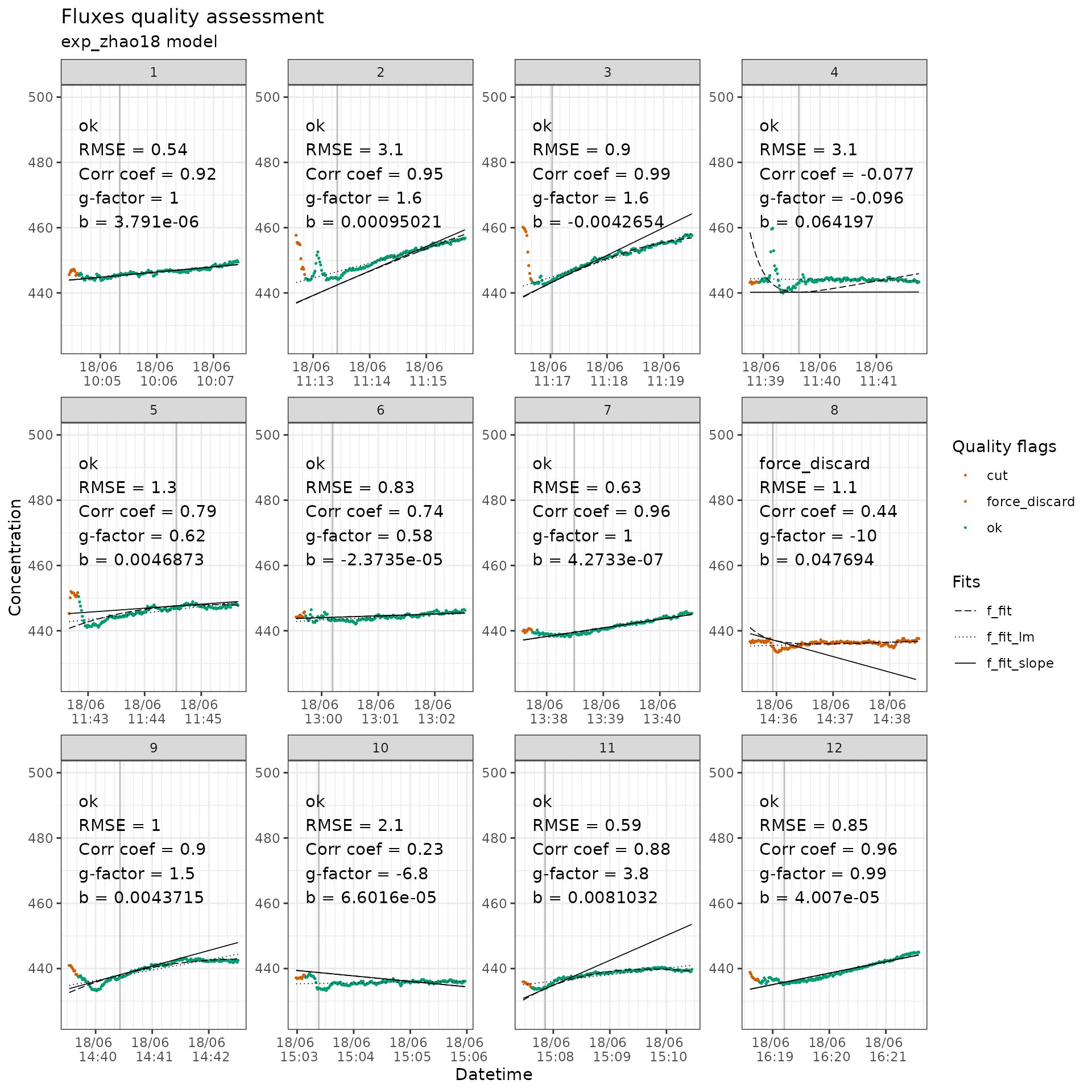
CO2 measurements with quality flags.
flag_twogases_ch4 |>
  flux_plot(
    f_conc = ch4_conc,
    f_datetime = datetime,
    f_ylim_upper = 2000,
    f_ylim_lower = 1995,
    y_text_position = 1997
  )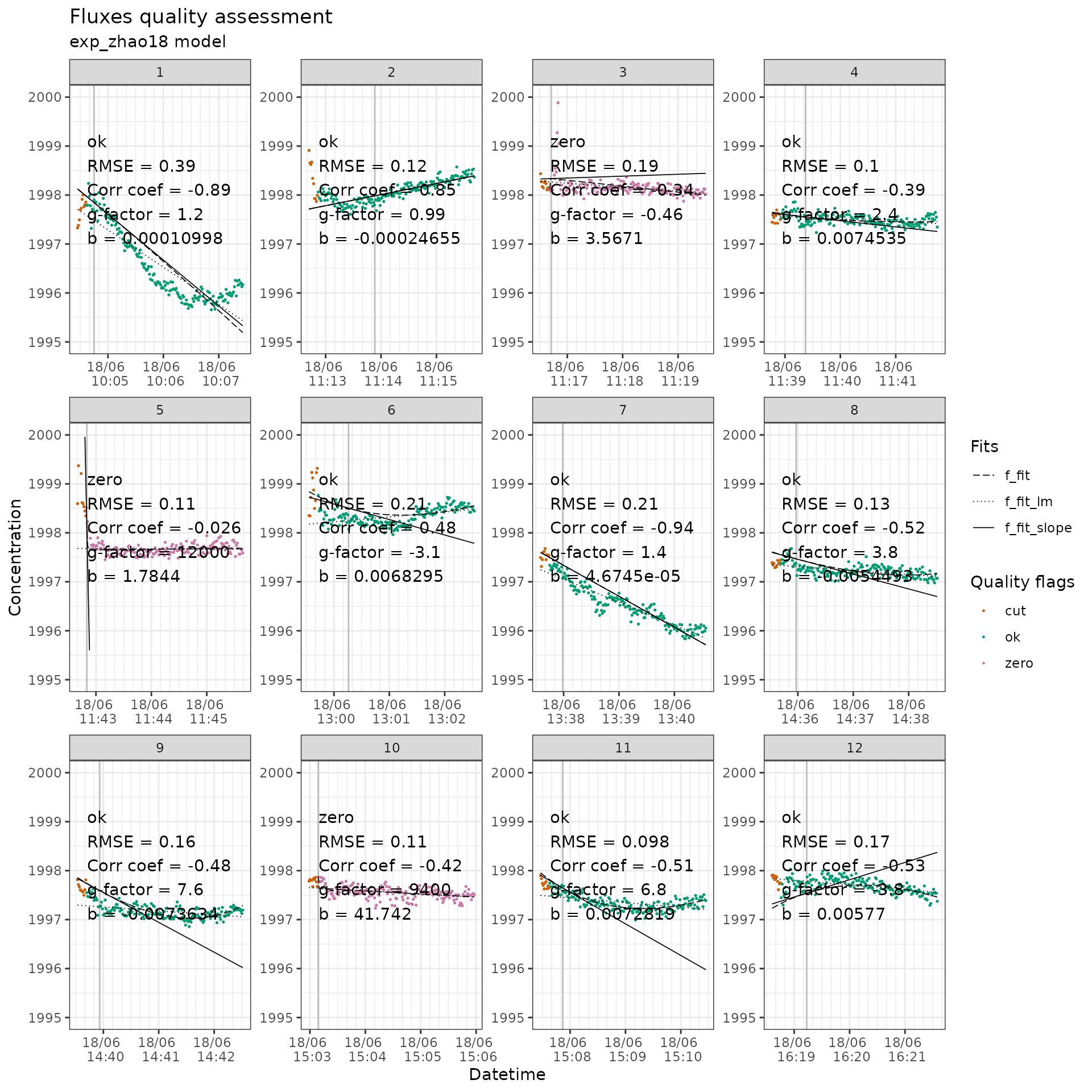
CH4 measurements with quality flags.
After calculating the fluxes, we need to rename the
f_flux column to avoid confusion when joining the
datasets:
fluxes_twogases_co2 <- flux_calc(
  slopes_df = flag_twogases_co2,
  slope_col = f_slope_corr,
  f_datetime = datetime,
  temp_air_col = temp_air,
  conc_unit = "ppm",
  flux_unit = "mmol/m2/h",
  setup_volume = 6.31,
  atm_pressure = 1,
  plot_area = 0.31,
  # we want to use the quality flags of CO2 to eventally discard CH4 fluxes
  cols_keep = "f_quality_flag"
) |>
  rename( # to avoid any confusion, we rename the flux column
    flux_co2 = "f_flux"
  ) |> # and we remove the slope one
  select(-f_slope_corr)

fluxes_twogases_ch4 <- flux_calc(
  slopes_df = flag_twogases_ch4,
  slope_col = f_slope_corr,
  f_datetime = datetime,
  temp_air_col = temp_air,
  conc_unit = "ppb", # ch4 is measured in ppb
  flux_unit = "umol/m2/h", # we want a flux in umol/m2/h
  setup_volume = 6.31,
  atm_pressure = 1,
  plot_area = 0.31
) |>
  rename( # to avoid any confusion, we rename the flux column
    flux_ch4 = "f_flux"
  ) |> # and we remove the slope one
  select(-f_slope_corr)
Then we can join the datasets. If the final dataset ends up being
longer, it probably means that some values in columns that should be
equal (f_temp_air_ave for example) are in fact not equal,
which leads to additional rows when joining the dataframes.
fluxes_twogases <- left_join(
  fluxes_twogases_co2,
  fluxes_twogases_ch4,
  by = c(
    # if that does not work, then it means that we did
    # something different for one of the gases
    "f_fluxid",
    "f_temp_air_ave",
    "datetime",
    "f_model"
  )
) |>
  mutate( # we discard the CH4 fluxes based on CO2 fluxes quality flags
    flux_ch4 = case_when(
      f_quality_flag %in% c("discard", "force_discard") ~ NA,
      .default = flux_ch4
    )
  )
Structure of fluxes_twogases:
#> tibble [12 × 7] (S3: tbl_df/tbl/data.frame)
#>  $ f_quality_flag: chr [1:12] "ok" "ok" "ok" "ok" ...
#>  $ f_fluxid      : Factor w/ 12 levels "1","2","3","4",..: 1 2 3 4 5..
#>  $ f_temp_air_ave: num [1:12] 13.4 16.5 17.1 14.4 15 ...
#>  $ datetime      : POSIXct[1:12], format: "2024-06-18 10:04:37" ...
#>  $ flux_co2      : num [1:12] 0.08292 0.38505 0.43518 0.00108 0.0637..
#>  $ f_model       : chr [1:12] "exp_zhao18" "exp_zhao18" "exp_zhao18"..
#>  $ flux_ch4      : num [1:12] -0.04873 0.01165 0 -0.00649 0 ...
In this example we calculated the fluxes for two gases measured
simultaneously by repeating the process for each gas, and in the end we
joined them and applied a rule that discarded the fluxes of one gas
based on the quality flags of the other. It is of course totally
possible to apply other rules, or to just keep the fluxes as provided by
fluxible.