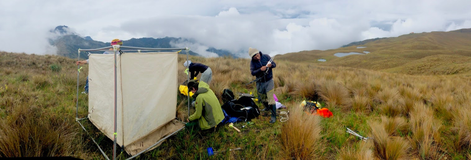
This vignette shows how to process ecosystem fluxes (CO2 and H2O) measured with the LI7500 tent setup presented in Halbritter et al. (2024). Because of field constraints, this setup differs from the smaller chamber in several points:
- one file per flux
- start and end of files do not represent start and end of measurements because setting up the tent can take more or less time
- for similar reasons, the length of the measurements is not constant
Importing the files
We import the data with licoread::import7500.
library(licoread)
li7500_data <- import7500(
  "ex_data/li7500",
  plotinfo = c("site", "treatment", "date", "plot_id", "trial")
)
The licoread::import7500 function provides
f_start and f_end, meaning we could skip
fluxible::flux_match. However, f_start and
f_end are based on the start and end of the files, which
would require a strict data collection routine. If such a strict routine
did not happen, there are two options to deal with that.
Making a new field record
If f_start and f_end cannot be used as
start and end of measurement, we can recreate a record file (for example
in a spreadsheet) with the real start and end datetime:
- use start and end from
licoread::import7500 - process fluxes until visualization (
flux_fitting,flux_qualityandflux_plot) - based on the plots, create a
recordfile with metadata identifying the fluxes (filename), start and end (note thatflux_matchrequires datetime format) - rename the columns
f_start,f_endandf_fluxidto avoid losing those informations (flux_matchwill overwrite them) - include
flux_matchbeforeflux_fittingin your workflow, and match the fluxes with the record file you created - adapt the record file if necessary and rerun until
flux_plot - once satisfied with cutting and fitting, run
flux_calcas normally
That makes the processing non homogeneous but still reproducible.
One side is reliable
If the start or the end are consistent but not the other, you can
change the direction of the cutting in flux_fitting. By
default, flux_fitting cuts the focus window as
start + start_cut to end - end_cut. The
argument cut_direction allows to change that:
-
cut_direction = "from_start"means the focus window will be fromstart + start_cuttostart + end_cut -
cut_direction = "from_end"means the focus window will be fromend - start_cuttoend - end_cut
Processing with fluxible
CO2
Wet air correction:
library(fluxible)
li7500_data_co2 <- flux_drygas(li7500_data, `CO2 umol/mol`, `H2O mmol/mol`)
Fitting a linear model:
li7500_fits_co2 <- flux_fitting(li7500_data_co2,
                                f_conc = `CO2 umol/mol_dry`,
                                fit_type = "linear")
Using fluxible::flux_quality to assess the quality of
the dataset.
li7500_flags_co2 <- flux_quality(li7500_fits_co2,
                                 f_conc = `CO2 umol/mol_dry`,
                                 rsquared_threshold = 0.5)
#>
#>  Total number of measurements: 4
#>
#>  ok   4   100 %
#>  discard      0   0 %
#>  zero     0   0 %
#>  force_discard    0   0 %
#>  start_error      0   0 %
#>  no_data      0   0 %
#>  force_ok     0   0 %
#>  force_zero   0   0 %
#>  force_lm     0   0 %
#>  no_slope     0   0 %
Plotting:
flux_plot(li7500_flags_co2,
          f_conc = `CO2 umol/mol_dry`,
          f_ylim_upper = 500,
          y_text_position = 450,
          print_plot = TRUE)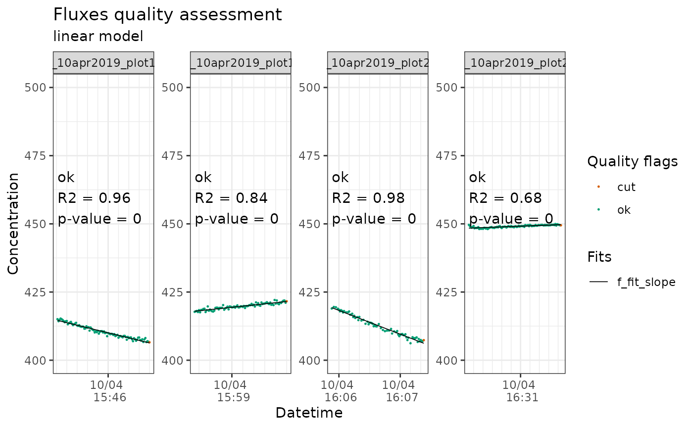
Output of flux_plot for CO2 fluxes
Can be exported in pdf directly (much easier to handle with a lot of data) with:
flux_plot(li7500_flags_co2,
          f_conc = `CO2 umol/mol_dry`,
          f_ylim_upper = 500,
          y_text_position = 450,
          print_plot = FALSE,
          output = "longpdf",
          f_plotname = "li7500_co2")
If other data (PAR and co) need processing, that would happen here.
To “compress” environmental variables at a single value per flux, see
the arguments cols_ave, cols_sum, and
cols_med in fluxible::flux_calc. To keep the
raw data (gas concentration or anything else) in a nested column, see
the cols_nest argument.
Now let’s calculate the fluxes with
fluxible::flux_calc.
li7500_fluxes_co2 <- flux_calc(li7500_flags_co2,
                               slope_col = f_slope_corr,
                               temp_air_col = Temperature,
                               setup_volume = 2197,
                               atm_pressure = pressure_atm,
                               plot_area = 1.44,
                               conc_unit = "ppm",
                               flux_unit = "umol/m2/s",
                               cols_keep = c(
                                 "site", "treatment", "date", "plot_id", "trial"
                               ))
#> Cutting data according to 'keep_arg'...
#> Averaging air temperature for each flux...
#> Creating a df with the columns from 'cols_keep' argument...
#> Calculating fluxes...
#> Concentration was measured in ppm
#> R constant set to 0.082057 L * atm * K^-1 * mol^-1
#> Fluxes are in umol/m2/sH2O
Wet air correction:
li7500_data_h2o <- flux_drygas(li7500_data, `H2O mmol/mol`, `H2O mmol/mol`)Fitting a linear model:
li7500_fits_h2o <- flux_fitting(li7500_data_h2o,
                                f_conc = `H2O mmol/mol_dry`,
                                fit_type = "linear",
                                start_cut = 0,
                                end_cut = 0)
Using fluxible::flux_quality to assess the quality of
the dataset:
li7500_flags_h2o <- flux_quality(li7500_fits_h2o,
                                 f_conc = `H2O mmol/mol_dry`,
                                 rsquared_threshold = 0.5,
                                 ambient_conc = 10, # the default is for CO2
                                 error = 2)
#>
#>  Total number of measurements: 4
#>
#>  ok   4   100 %
#>  discard      0   0 %
#>  zero     0   0 %
#>  force_discard    0   0 %
#>  start_error      0   0 %
#>  no_data      0   0 %
#>  force_ok     0   0 %
#>  force_zero   0   0 %
#>  force_lm     0   0 %
#>  no_slope     0   0 %
Plotting:
flux_plot(li7500_flags_h2o,
          f_conc = `H2O mmol/mol_dry`,
          print_plot = TRUE,
          f_ylim_lower = 5,
          f_ylim_upper = 15,
          y_text_position = 12)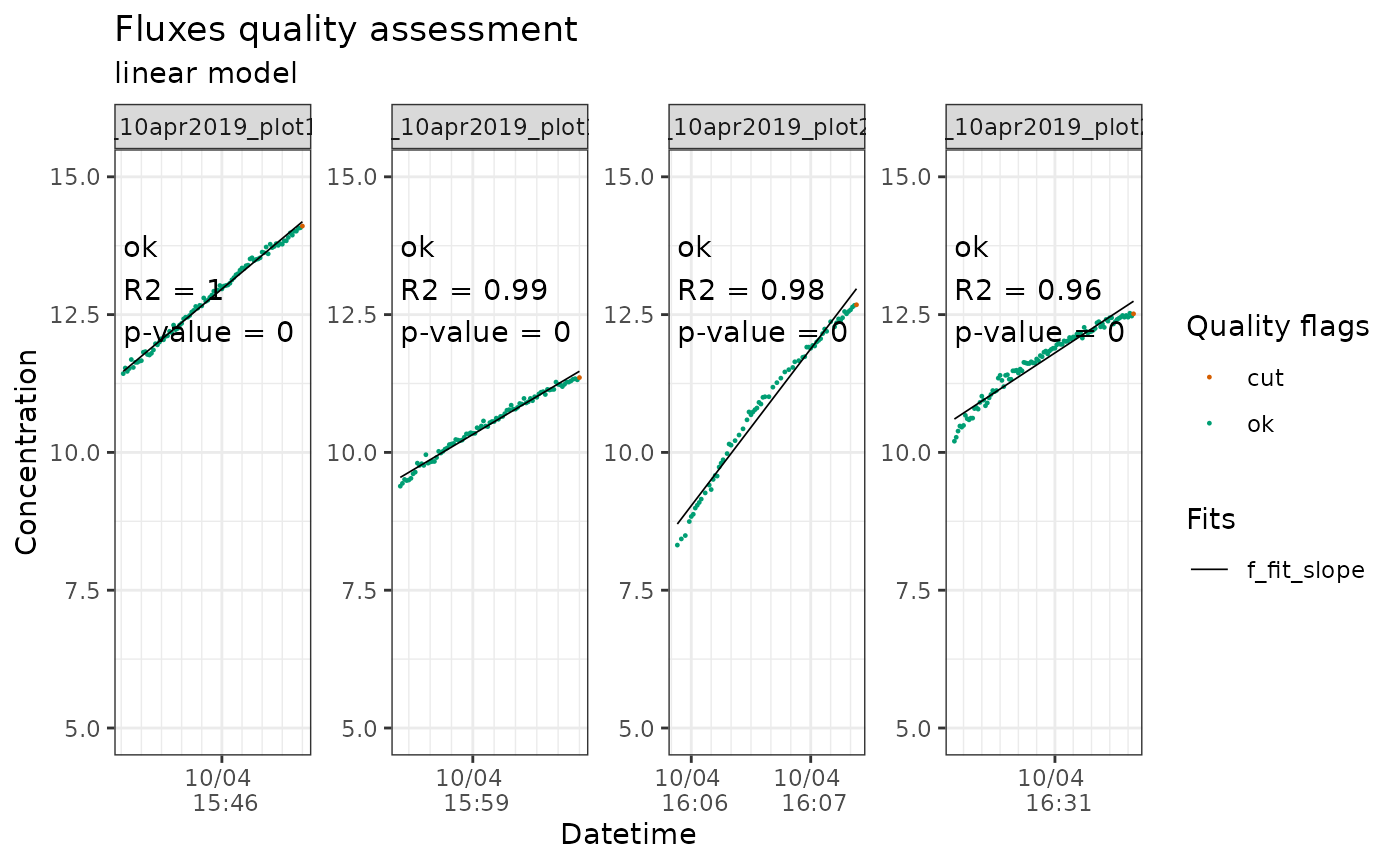
Output of flux_plot for H2O fluxes
Or directly exported as a pdf:
flux_plot(li7500_flags_h2o,
          f_conc = `H2O mmol/mol_dry`,
          print_plot = FALSE,
          output = "longpdf",
          f_plotname = "li7500_h2o",
          f_ylim_lower = 5,
          f_ylim_upper = 15,
          y_text_position = 12)
Flux calculations:
li7500_fluxes_h2o <- flux_calc(li7500_flags_h2o,
                               slope_col = f_slope_corr,
                               temp_air_col = Temperature,
                               setup_volume = 2197,
                               atm_pressure = pressure_atm,
                               plot_area = 1.44,
                               conc_unit = "mmol/mol",
                               flux_unit = "mmol/m2/s",
                               cols_keep = c(
                                 "site", "treatment", "date", "plot_id", "trial"
                               ))
#> Cutting data according to 'keep_arg'...
#> Averaging air temperature for each flux...
#> Creating a df with the columns from 'cols_keep' argument...
#> Calculating fluxes...
#> Concentration was measured in mmol/mol
#> R constant set to 0.082057 L * atm * K^-1 * mol^-1
#> Fluxes are in mmol/m2/s
Calculating Gross Primary Production and Transpiration
I’m glad you asked! The function fluxible::flux_diff is
precisely made for that.
Further calculations
In order to calculate carbon and water use efficiencies, we need both H2O and CO2 fluxes in the same dataset.
library(tidyverse)
# to avoid confusion, we add a gas column
# this might be implemented in flux_calc in the future

li7500_fluxes_co2 <- li7500_fluxes_co2 |>
  mutate(gas = "co2")

li7500_fluxes_h2o <- li7500_fluxes_h2o |>
  mutate(gas = "h2o")

li7500_fluxes <- bind_rows(li7500_fluxes_co2, li7500_fluxes_h2o)

# Now the data are in a single long df
#> tibble [12 × 13] (S3: tbl_df/tbl/data.frame)
#> $ trial : chr [1:12] "GPP" "p" "r" "GPP" ...
#> $ f_flux : num [1:12] -5.59 -3.83 1.76 -6.52 -5.98 ...
#> $ f_fluxid : chr [1:12] "ACJ_C_10apr2019_plot1_p.txt" "AC"..
#> $ f_slope_corr : num [1:12] -0.0927 -0.0927 0.0424 -0.1442 -0...
#> $ f_temp_air_ave : num [1:12] 25.6 25.6 25 24.8 24.8 ...
#> $ f_atm_pressure_ave: num [1:12] 0.664 0.664 0.665 0.664 0.664 ...
#> $ f_datetime : POSIXct[1:12], format: "2019-04-10 15:45:11" ..
#> $ f_model : chr [1:12] "linear" "linear" "linear" "linea"..
#> $ site : chr [1:12] "ACJ" "ACJ" "ACJ" "ACJ" ...
#> $ treatment : chr [1:12] "C" "C" "C" "C" ...
#> $ date : chr [1:12] "10apr2019" "10apr2019" "10apr201"..
#> $ plot_id : chr [1:12] "plot1" "plot1" "plot1" "plot2" ...
#> $ gas : chr [1:12] "co2" "co2" "co2" "co2" ...